Principles & Metrics of Jitter and Wander

Technical article

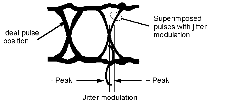
Jitter and wander are defined respectively as "the short-term and the long-term variations of the significant instants of a digital signal from their ideal positions in time". One way to think of this is a digital signal continually varying its position in time by moving backwards and forwards with respect to an ideal clock source. Most engineers' first introduction to jitter is viewed on an oscilloscope (Figure 1). When triggered from a stable reference clock, jittered data is clearly seen to be moving in relation to a reference clock.

Figure 1. Jitter as viewed on an oscilloscope

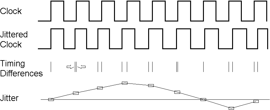
In fact, jitter and wander on a data signal are equivalent to a phase modulation of the clock signal used to generate the data (Figure 2). Naturally, in a practical situation, jitter will be composed of a broad range of frequencies at different amplitudes.

Figure 2. Phase variation between two signals

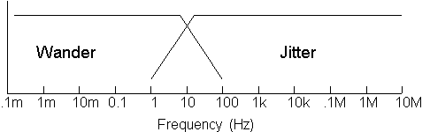
Jitter and wander have both an amplitude: how much the signal is shifting in phase - and a frequency: how quickly the signal is shifting in phase. Jitter is defined in the ITU-T G.810 standard as phase variation with frequency components greater than or equal to 10 Hz whilst wander is defined as phase variations at a rate less than 10 Hz (Figure 3).

Figure 3. Frequency ranges of jitter and wander (ref. G.810)

When measuring jitter or wander, always be sure what the reference clock is. By definition, a signal has no phase variation when referenced to itself - jitter or wander always refers to a difference between one timed signal and another.

Metrics for Jitter

Jitter is normally specified and measured as a maximum phase amplitude within one or more measurement bandwidths. A single interface may be specified using several different bandwidths since the effect of jitter varies depending on its frequency, as well as its amplitude.

UI (Unit Intervals)

Jitter amplitude is specified in Unit Intervals (UI), such that one UI of jitter is equal to one data bit-width, irrespective of the data rate. For example, at a data rate of 2048 kbit/s, one UI is equivalent to 488 ns, whereas at a data rate of 155.52 Mbit/s, one UI is equivalent to 6.4 ns.

Jitter amplitude is normally quantified as a Peak-to-Peak value rather than an RMS value, since it is the peak jitter that would cause a bit error to be made in network equipment.

However, RMS values are useful for characterising or modelling jitter accumulation in long line systems using SDH regenerators, for example, and the appropriate specifications use this metric instead of Peak-to-Peak.

Metrics for Wander

A wander measurement requires a "wander-free" reference, relative to which the wander of another signal is measured. Any Primary Reference Clock (PRC) can serve as a reference because of its long-term accuracy (10–11 or better) and good short-term stability. A PRC is usually realised with a caesium-based clock, although it may also be realised using GPS technology.

Because it involves low frequencies with long periods, wander data can consist of hours of phase information. However, because phase transients are of importance, high temporal resolution is also needed. So to provide a concise measure of synchronisation quality, three wander parameters have been defined and are used to specify performance limits:

• TIE Time Interval Error (wander in ns)
• MTIE Maximum Time Interval Error (related to Peak-to-Peak wander)
• TDEV Time Deviation (related to rms wander)

Formal mathematical definitions of these and other parameters can be found in ITU-T G.810 standard.

TIE (Time Interval Error)

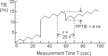
TIE is defined as the phase difference between the signal being measured and the reference clock, typically measured in ns. TIE is conventionally set to zero at the start of the total measurement period T. Therefore TIE gives the phase change since the measurement began. An example is given in Figure 4. The increasing trend shown is due to a frequency offset of about 1 ns per 10 s, or 10–10 in this case.

Figure 4. Example of TIE wander measurement

MTIE (Maximum Time Interval Error)

MTIE is a measure of wander that characterises frequency offsets and phase transients. It is a function of a parameter t called the Observation Interval. The definition (Figure 5) is:

MTIE(t) is the largest Peak-to-Peak TIE (i.e.,. wander) in any observation interval of length t.

Figure 5. Functional definition of MTIE

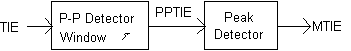
In order to calculate MTIE at a certain observation interval t from the measurement of TIE, a time window of length t is moved across the entire duration of TIE data, storing the peak value. The peak value is the MTIE(t) at that particular t. This process is repeated for each value of t desired.

For example, Figure 4 shows a window of length t=20 sec at a particular position. The Peak-to-Peak TIE for that window is 4 ns. However, as the 20 sec window is slid through the entire measurement period, the largest value of ppTIE is actually 11 ns (at about 30 sec into the measurement).

Therefore MTIE(20 s) = 11 ns.

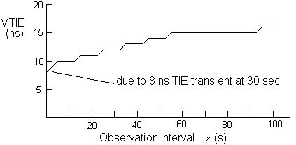
Figure 6 shows the complete plot of MTIE(t) corresponding to the plot of TIE in Figure 4. The rapid 8 ns transient at t = 30 s is reflected in the value MTIE(t) = 8 ns for very small t.

It should be noted that the MTIE plot is monotonically increasing with observation interval and that the largest transient masks events of lesser amplitude.

Figure 6. Example of MTIE wander measurement (corresponding to Figure 4)

TDEV (Time Deviation)

TDEV is a measure of wander that characterises its spectral content. It is also a function of the parameter t called Observation Interval. The definition (Figure 7) is:

TDEV(t) is the rms of filtered TIE, where the bandpass filter (BPF) is centred on a frequency of 0.42/t.

Figure 7. Functional definition of TDEV

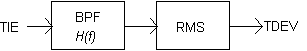
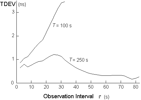
Figure 8 shows two plots of TDEV(t). The first plot (for T=100s), corresponding to the TIE data of Figure 4 shows TDEV rising with t. This is because, for the short measurement period T=100s, the two transients in Figure 4 dominate.

If we were to make a longer TIE measurement out to T = 250s, the effect of the two transients on TDEV would become less, assuming there are no more transients. The TDEV characteristic labelled T=250 s would be the result.

It should also be noted that TDEV is insensitive to constant phase slope (frequency offset).

To calculate TDEV for a particular t, the overall measurement period T must be at least 3t. For an accurate measure of TDEV, a measurement period of at least 12t is required. This is because the rms part of the TDEV calculation requires sufficient time to get a good statistical average.

Figure 8. Example of TDEV wander measurement (corresponding to Figure 4)

Acronyms

3/97