This example shows how the software supports the analytical method of finding process bottlenecks, determining process throughput, and balancing resources. This section requires running the actual software.
This section guides the user through the following steps:
From this point on, you must run the actual software. Make sure the two software packages (Process Modeling software and Simulation software) have been successfully installed before proceeding. Please read the release notes and follow the installation instructions for the two software packages. Solutions to common installation problems are presented at the end of this chapter in the trouble shooting guide.
Opening and reviewing the order processing model
Let's open the Process Modeling software model that represents the order processing example and export it to Simulation software. To do so:
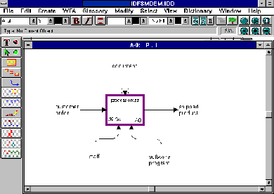
The context page (A-0) is the current page. This page shows that the process order system receives as input customer orders and produces Shipped Orders using staff and software programs to do so. Process order has a decomposition page. To access it:
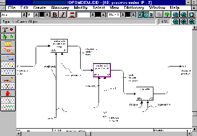
The A0 decomposition page opens:
This page shows three activities:
A1: receive order and generate image. When a customer order arrives, it is handled by a mailclerk who generates an electronic version of the order by means of a scan program.
A2: review and process order. The new electronic order form is reviewed and further processed by a dataentry clerk using the excel software. Details of how this processing is done are shown in the decomposition page for A2.
A3: ship order. When the order details have been entered, the order can be shipped. A shipper receives the order details and ships the product.
Let's now proceed with saving the diagram in a form that is suitable for importing in the Simulation software application, where we can conduct our analysis.
View the results of the simulation
When the simulation ends, the Simulation Complete window appears.
The results file opens.
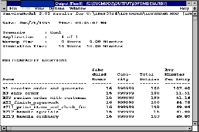
It contains summary statistics which cover activity and resource utilization. Notice that simulation time was sixteen hours and eighteen minutes. The required staffing should process that volume in less than two business days (fifteen hours). To determine what is preventing the processing from completing earlier, let's analyze the results.
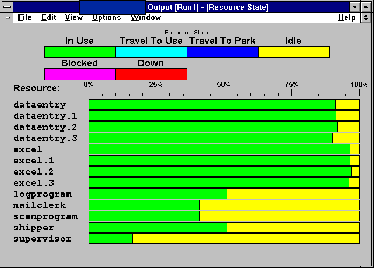
This chart shows all the resources that were utilized in this simulation run. For all resources it displays the percentage of time that resource is In Use or is Idle.
Let's now analyze only the utilization of the excel program. Notice that there are bars for excel.1, excel.2, excel.3 and excel. The ones numbered 1 through 3 represent the individual excel resources. The bar labeled excel only represents an average of the three excel resources used.
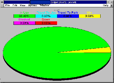
A pie graph of the average utilization of the 3 excel resources that were made available in this scenario appears. Notice that In Use is almost 100%.
The Duration Histogram Window appears now with 10 Histogram bars.
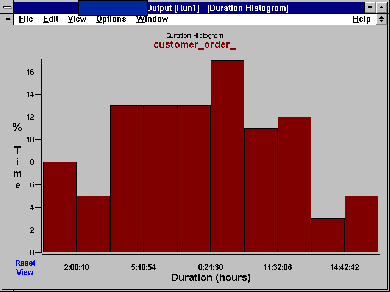
Notice the peak of 18% approximately nine hours into the run.
The Select window appears. This window lets you select which activities you want to include in your Content History Chart.
This chart shows the amount of work waiting to be processed at each activity location.
The Content History chart leaves only the plot lines for the activity A1.
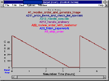
This chart is showing the work load at the A1 activity. Notice the peak of 50 jobs in coincidence with the arrival of the workload and the decrease thereafter.
From the observation of the resource state, a hypothesis can be made that more dataentry and excel resources are needed to complete the processing in time. Even though the biggest bottleneck is the excel resource, it is unlikely that the processing goals can be met by adding only more software, that is, an additional excel software program.